728x90
Scikit-Learn으로 머신러닝 모델 만들기
Scikit-Learn?
- 머신러닝 알고리즘을 구현한 오픈소스 라이브러리
- 알고리즘: Pyhton Class
- 데이터 셋: Numpy 배열, Pandas에서 제공하는 DataFrame, SciPy에서 제공하는 희소행렬
Scikt-Learn algorithm cheat-sheet
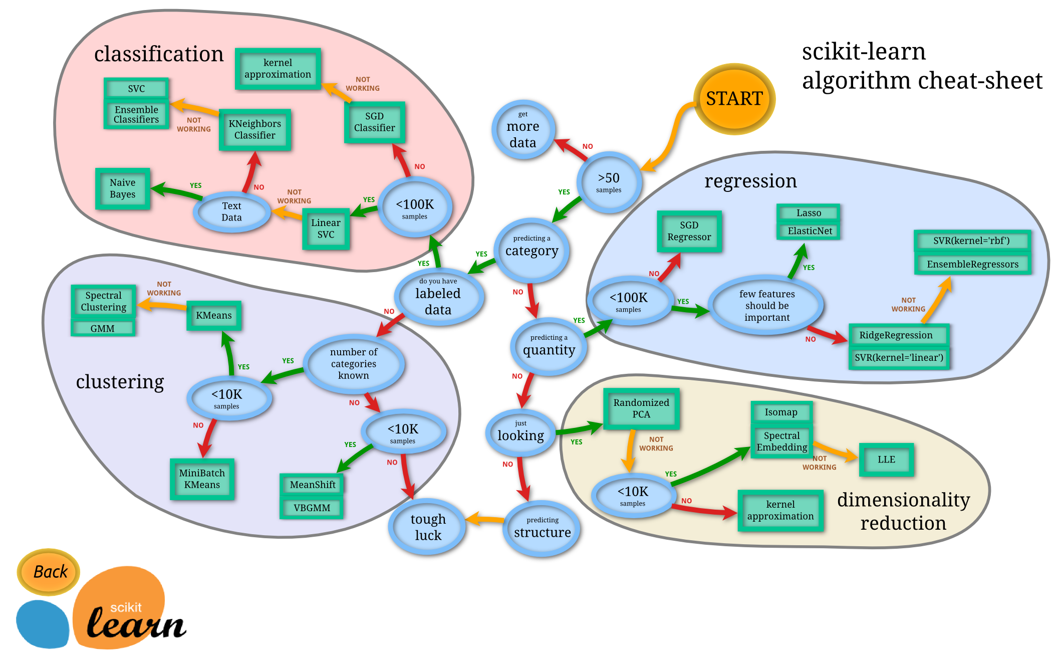
Scikit-Learn 치트시트는 알고리즘을 어떤 것으로 사용할지 고민될 때 매우 유용하다.
Start → 샘플의 개수가 50개 이상인가? → Yes/No → Yes: 오케이! 그럼 분류문제인지 수치문제인지?/No:그럼 데이터 더 모아와! → Yes: 분류문제/No: 수치문제 → 분류문제인 경우, 라벨링 여부 Yes/No → Yes: 지도학습(Classification), 비지도학습(Clustering)/No: regression, dimensionality reduction ... 이런식으로 시트를 따라가다 보면 데이터에 적합한 알고리즘을 찾을 수 있다.
Scikit-Learn에는 웬만한 샘플 데이터들이 포함되어 있다. 데이터 표현 방식으로는 특징 행렬(Feature Matrix)와 대상 벡터(Target Vector)가 있다.
- 특징 행렬(Feature Matrix): 표본(sample)-특징(feature), 행의 개수 ->n_samples, 열의 개수->n_features, 특징 행렬은 변수 X에 저장, [n_samples, n_features]형태의 2차원 배열 구조(Numpy 배열, Pandas DataFrame, Scipy 희소 행렬 사용)
- 대상 벡터(Target Vector): 연속적인 수치값, 이산 클래스와 레이블, 길이->n_samples, 대상벡터는 변수 y에 저장, 1차원 배열 구조(Numpy 배열, Pandas Series 사용), 특징 행렬로부터 예측하고자 하는 값의 벡터, 종속/출력/결과/반응 변수라고도 함
Scikit-Learn에서 제공하는 iris 데이터셋을 이용하여 머신러닝 모델을 만들어 보자.
# iris 데이터 불러오기
from sklearn.datasets import load_iris

# 변수에 데이터 저장
iris_dataset = load_iris()

# 데이터 타입 확인
print(type(iris_dataset['data']))

》<class 'numpy.ndarray'> # iris 데이터는 넘파이 배열로 되어 있다.

#Description 확인
# 배열로 가져오기:
iris_dataset['DESCR']

# 속성으로 가져오기:
iris_dataset.DESCR
# 배열로 가져오든 속성으로 가져오든 결과는 똑같다.

》.. _iris_dataset:\n\nIris plants dataset\n--------------------\n\n**Data Set Characteristics:**\n\n :Number of Instances: 150 (50 in each of three classes)\n :Number of Attributes: 4 numeric, predictive attri... 블라블라

# key를 확인해 보자.
print('iris_dataset의 키:\n', iris_dataset.keys())
》iris_dataset의 키:
dict_keys(['data', 'target', 'frame', 'target_names', 'DESCR', 'feature_names', 'filename', 'data_module'])
#라벨은 target에 들어있다.

# target names를 확인해 보자.
print('타깃의 이름: \n', iris_dataset['target_names'])

》타깃의 이름:
['setosa' 'versicolor' 'virginica']

# features names를 확인해 보자.
print('특징의 이름: \n', iris_dataset['feature_names'])

》특징의 이름:
['sepal length (cm)', 'sepal width (cm)', 'petal length (cm)', 'petal width (cm)']
# sepal 꽃받침, petal 꽃잎

# 데이터의 크기를 확인해 보자.
print(iris_dataset['data'].shape)

》(150, 4) #2차원 데이터

# 데이터 처음~5번째까지만 확인해 보자.
print(iris_dataset['data'][:5])

》[[5.1 3.5 1.4 0.2] [4.9 3. 1.4 0.2] [4.7 3.2 1.3 0.2] [4.6 3.1 1.5 0.2] [5. 3.6 1.4 0.2]]

# target의 크기를 확인해 보자.
print(iris_dataset['target'].shape)

》(150,) # 1차원 데이터

# target의 내용을 확인해 보자.
print(iris_dataset['target'])

》[0 0 0 0 0 0 0 0 0 0 0 0 0 0 0 0 0 0 0 0 0 0 0 0 0 0 0 0 0 0 0 0 0 0 0 0 0 0 0 0 0 0 0 0 0 0 0 0 0 0 1 1 1 1 1 1 1 1 1 1 1 1 1 1 1 1 1 1 1 1 1 1 1 1 1 1 1 1 1 1 1 1 1 1 1 1 1 1 1 1 1 1 1 1 1 1 1 1 1 1 2 2 2 2 2 2 2 2 2 2 2 2 2 2 2 2 2 2 2 2 2 2 2 2 2 2 2 2 2 2 2 2 2 2 2 2 2 2 2 2 2 2 2 2 2 2 2 2 2 2]

# setosa 0
# versicolor 1
# virginica 2

#학습시킬 데이터 준비하기
from sklearn.model_selection import train_test_split

# 학습용 데이터(X_train)와 테스트용 데이터(X_test)를 쪼개준다.
# feature: X_train, X_test
# label: Y_train, Y_test
# → 총 4조각의 데이터 필요

# 요구사항: data를 훈련 데이터로 사용, target을 레이블로 사용, random 값 주기: 반복시 동일한 결과 도출
train_test_split(iris_dataset['data'],iris_dataset['target'], random_state=0)

# 'X_train, X_test, y_train, y_test' 변수에 저장
X_train, X_test, y_train, y_test = train_test_split(iris_dataset['data'],iris_dataset['target'], random_state=0)

# 쪼갠 데이터의 크기를 확인해 보자.
# 학습용 데이터
print('X_train 크기:', X_train.shape)
print('y_train 크기:', y_train.shape)

≫
X_train 크기: (112, 4)
y_train 크기: (112,)

# 테스트용 데이터
print('X_test 크기:', X_test.shape)
print('y_test 크기:', y_test.shape)

≫
X_train 크기: (38, 4)
y_train 크기: (38,)
# test 데이터 비율이 너무 작다! random_state=0 옆에 test_size=0.5를 추가해 준다. 그럼 5:5 비율로 쪼개진다. 7:3정도가 적당하므로 test_size=0.3으로 수정한다.

# 수정 후 학습용 데이터
print('X_train 크기:', X_train.shape)
print('y_train 크기:', y_train.shape)

≫
X_train 크기: (105, 4)
y_train 크기: (105,)

# 수정 후 테스트용 데이터
print('X_test 크기:', X_test.shape)
print('y_test 크기:', y_test.shape)

≫
X_train 크기: (45, 4)
y_train 크기: (45,) # 여기까지 데이터 준비 끝.

# 데이터 시각화하기
import pandas as pd
import matplotlib .pyplot as plt

# 데이터 프레임객체로 만들기
# 계속 사용할 것이므로 변수에 저장
iris_dataframe = pd.DataFrame(X_train, columns=iris_dataset['feature_names'])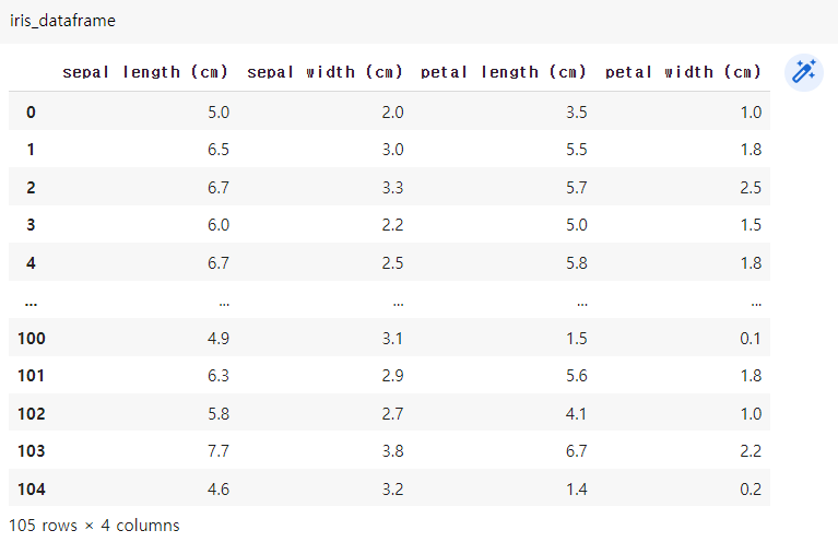
# 데이터 예쁘게 만들기(시각화)
pd.plotting.scatter_matrix(iris_dataframe)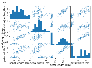
# scatter_matrix는 여러개를 한꺼번에 보여줄 때 사용
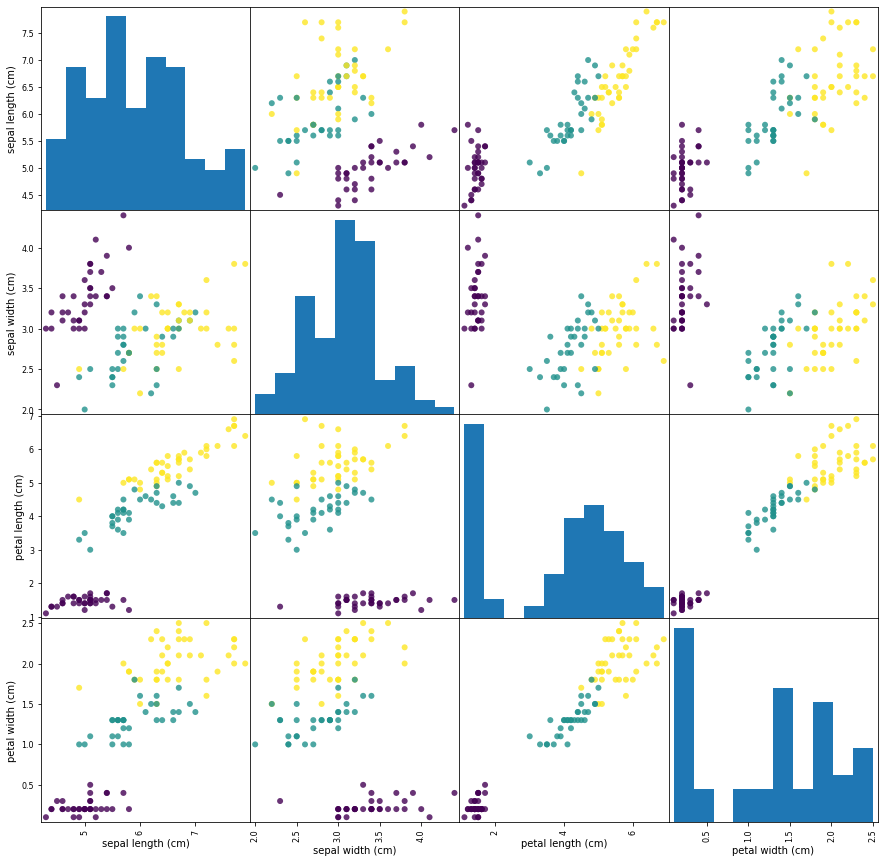
# 더 보기 좋게 만들어 보자.
pd.plotting.scatter_matrix(iris_dataframe, figsize=(15,15),
marker='o',
c=y_train,
cmap='viridis',
alpha=0.8)
# figsize: 그림판 크기
# marker: 점 어떻게 표현할 것인지
# c: 색상값 지정(라벨인 y_train으로 지정)
# cmap: 색상 지정
# alpha: 알파값 지정(투명0.0~불투명1.0 사이의 값)
# 머신러닝 모델 만들기: k-최근접 알고리즘
# Classifier(분류)와 Regressor(예측) 중에 고를 수 있다. 꽃을 분류할 것이므로 Classifier 선택
from sklearn.neighbors import KNeighborsClassifier
knn = KNeighborsClassifier(n_neighbors=1)
# n_neighbors=1 주변에 몇 개를 가지고 판단할 것인지 설정

# 학습시키기
knn.fit(X_train, y_train) # 학습 결과는 knn에 들어간다.

# 테스트하기
# 2차원 데이터를 하나 만든다. 꽃받침의 길이와 넓이, 꽃잎의 길이와 넓이
import numpy as np
X_new = np.array([[5, 2.9, 1, 0.2]])

# 예측하기
knn.predict(X_new)

≫ array([0]) # 0번은 setosa. 위의 데이터가 setosa라고 예측함

# 0: setosa
# 1: versicolor
# 2: virginica

# 테스트(예측)하여 나온 값을 보기 좋게 만들어 보자.
prediction = knn.predict(X_new)
print('예측:', prediction)
print('예측한 타깃의 이름:', iris_dataset['target_names'][prediction])

≫
예측: [0]
예측한 타깃의 이름: ['setosa']

# 모델 평가하기
y_pred = knn.predict(X_test)
print(y_pred)

≫ [2 1 0 2 0 2 0 1 1 1 2 1 1 1 1 0 1 1 0 0 2 1 0 0 2 0 0 1 1 0 2 1 0 2 2 1 0 2 1 1 2 0 2 0 0]

# y_pred(예측값)과 y_test(실측값) 비교하기
y_pred == y_test

≫ array([ True, True, True, True, True, True, True, True, True, True, True, True, True, True, True, True, True, True, True, True, True, True, True, True, True, True, True, True, True, True, True, True, True, True, True, True, True, False, True, True, True, True, True, True, True])
*False 하나 빼고 모두 True로 나왔으므로 정확도가 높다고 할 수 있다.

# 평균 내기
np.mean(y_pred == y_test)

≫ 0.9777777777777777
# 97%의 정확도를 가진 모델이다. 즉, 테스트 세트에 대한 정확도: 97.7%
iris dataset으로 머신러닝 모델 만들기 미션 complete!

728x90
'MS AI School' 카테고리의 다른 글
| DAY 20 - 머신러닝 지도 학습: 결정 트리 모델, SVM, 다중 MLP 회귀 (0) | 2022.11.23 |
|---|---|
| DAY 19 - 머신러닝 지도 학습: 선형 회귀 (0) | 2022.11.01 |
| DAY 15 - Feature와 Label, Data Preprocessing(데이터 전처리) (0) | 2022.11.01 |
| DAY 14 - Flask, Web crawling(BS4), MySQL (0) | 2022.11.01 |
| DAY 13 - Matplotlib (0) | 2022.11.01 |